Gradient Descent

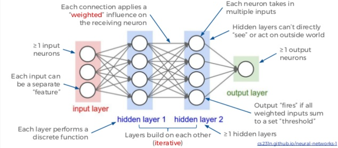
Neural Network as a Chain of Functions

To understand deep learning, we need to understand the concept of a neural network as a chain of functions.

A Neural Network is essentially a chain of functions. It consists of a set of inputs connected through ‘weights’ to a set of activation functions, whose output becomes the input for the next layer, and so on.

The Forward Pass

Let’s consider a simple two-layer neural network.

• $x$: Input vector
• $y$: Output vector (prediction)
• $L$: Number of layers
• $w^l, b^l$: Weights and biases for layer $l$
• $a^l$: Activation of layer $l$ (we use sigmoid $\sigma$ here)

The flow of data (Forward Pass) can be represented as:

For any layer $l$, the activation $a^l$ is calculated as:

where $a^0 = x$ (the input).

The linear transformation:

$z = w^T x + b$

defines a hyperplane (decision boundary) in the feature space.

The activation function then introduces non-linearity, allowing the network to combine multiple such hyperplanes into complex decision boundaries.

Why Non-Linearity Is Non-Negotiable

Without activation:

This collapses to:

Still one big linear transformation and hence one hyperplane; the problems of not able to separate features will come. Only because of non-linearity, we can get multiple hyperplanes and hence a composable complex decision boundaries that can separate features.

So the concept of Vectors, Matrices and Hyperplanes remain the same as before. Let us explore the chain of functions part here

A neural network with $L$ layers can be represented as a nested function:\(f(x) = f_L(...f_2(f_1(x))...)\)

Each “link” in the chain is a layer performing a linear transformation followed by a non-linear activation and cascading to the final output.

The Cost Function (Loss Function)

To train this network, we need to measure how “wrong” its predictions are compared to the true values. We do this using a Cost Function (or Loss Function).

A simplest Loss function is just the difference between the predicted output and the true output ($ y(x) - a^L(x) $.)

But usually we use the square of the difference to make it a non-negative function.

A common choice is the Mean Squared Error (MSE):

• $n$: Number of training examples
• $y(x)$: The true expected output (label) for input $x$
• $a^L(x)$: The network’s predicted output for input $x$

The Goal of Training

The goal of training is to find the set of weights $w$ and biases $b$ that minimize this cost $C$.

This means that we need to optimise each component of the function $f(x)$ to reduce the cost proportional to its contribution to the final output. The method to do this is called Backpropagation. It helps us calculate the gradient of the cost function with respect to each weight and bias.

Once the gradient is calculated, we can use Gradient Descent to update the weights in the opposite direction of the gradient.

Gradient descent is a simple optimization algorithm that works by iteratively updating the weights in the opposite direction of the gradient.

However neural network is a composition of vector spaces and linear transformations. Hence gradient descent acts on a very complex space.

There are two or three facts to understand about gradient descent:

1. It does not attempt to find the global minimum, but rather follows the local slope of the cost function and converges to a local minimum or a flat region. Saddle point is a good optimisation point.

2. Gradients can vanish or explode, leading to slow or unstable convergence. The practical solution to control this is to use learning rate and using adaptive learning rate methods like Adam or RMSprop.

3. Batch Size matters: Calculating the gradient over the entire dataset (Batch Gradient Descent) is computationally expensive and memory-intensive. In practice, we use Stochastic Gradient Descent (SGD) (one example at a time) or, more commonly, Mini-batch Gradient Descent (a small batch of examples). This introduces noise into the gradient estimate, which paradoxically helps the optimization process escape shallow local minima and saddle points.

Optimization: Gradient Descent — Take 1

Gradient Descent is a simple yet powerful optimization algorithm used to minimize functions by iteratively updating parameters in the direction that reduces the function’s output.

For basic scalar functions (e.g., $( f(x) = x^2 )$), the update rule is straightforward: \(x \leftarrow x - \eta \frac{df}{dx}\) where $( \eta )$ is the learning rate.

However, neural networks are not simple scalar functions. They are composite vector-valued functions — layers of transformations that take in high-dimensional input vectors and eventually output either vectors (like logits) or scalars (like loss values).

Understanding how to optimize these complex, high-dimensional functions requires us to extend basic calculus:

• The gradient vector helps when the function outputs a scalar but takes a vector input (e.g., a loss function w.r.t. weights).
• The Jacobian matrix becomes important when both the input and the output are vectors (e.g., when computing gradients layer by layer in backpropagation).

We’ll build up to this step by step — starting with scalar gradients, then moving to vector calculus, Jacobians, and how backpropagation stitches it all together.

Let’s take it one layer at a time.

Gradient Descent for Scalar Functions

Consider this simple system that composes two functions:

Where:

• $x$ is your input (fixed, given by your data)
• $w_1$ and $w_2$ are parameters you can adjust (like weights in a neural network)
• $f$ is the first function (think: first layer)
• $g$ is the second function (think: second layer)
• $L$ is the final output

Let’s make this concrete with simple linear functions:

\(f(x, w_1) = x \cdot w_1 + b_1\) \(g(z, w_2) = z \cdot w_2 + b_2\)

So the full composition is:

Running the Numbers: A Real Example

Let’s pick actual values and see what happens:

Fixed values:

• Input: $x = 2.0$
• Bias terms: $b_1 = 1.0$, $b_2 = 0.5$

Current parameter values:

• $w_1 = 0.5$
• $w_2 = 1.5$

Step 1: Compute intermediate result from first function:

Step 2: Compute final output from second function:

The problem: Suppose we want $L_{\text{target}} = 5.0$ instead!

Our current error is:

The million-dollar question: How should we change $w_1$ and $w_2$ to reduce this error?

The Adjustment Problem: Which Direction? How Much?

Here’s what we need to know:

1. Should we increase or decrease $w_1$? (Which direction?)
2. How sensitive is $L$ to changes in $w_1$? (How much?)
3. Same questions for $w_2$.

This is where derivatives come in! Specifically, we need:

These tell us:

• Sign: Positive means “increase $w$ increases $L$”, negative means the opposite

• Magnitude: Larger absolute value means $L$ is more sensitive to changes in $w$

But there’s a complication: $w_1$ doesn’t directly affect $L$. It affects $f$, which then affects $g$, which then affects $L$. This is a composition, and we need to trace the effect through multiple steps.

This is where the “Chain Rule” of Calculus comes into play.

The Chain of Effects

Let’s visualize how changes propagate:

Change w₁ → Affects f → Changes z → Affects g → Changes L
      ↓            ↓         ↓               ↓
      Δw₁        ∂f/∂w₁     Δz     ∂g/∂z     ΔL

Similarly for $w_2$ (but $w_2$ directly affects $g$):

Change w₂ → Affects g → Changes L
↓ ↓ ↓
Δw₂ ∂g/∂w₂ ΔL

The key insight: To find how $w_1$ affects $L$, we need to multiply the effects at each step.

This is the chain rule in action!

The Solution: Applying the Chain Rule

For our composition $L = g(f(x, w_1), w_2)$, let’s introduce a shorthand: call $z = f(x, w_1)$ the intermediate value.

Then:

Computing $\frac{\partial L}{\partial w_1}$:

By the chain rule of calculus:

Let’s compute each piece:

Part 1: How does $L$ change with $z$?

Part 2: How does $z$ change with $w_1$?

Putting it together:

Interpretation: If we increase $w_1$ by 0.1, then $L$ increases by approximately $3.0 \times 0.1 = 0.3$.

Computing $\frac{\partial L}{\partial w_2}$:

This is simpler because $w_2$ directly affects $g$:

Interpretation: If we increase $w_2$ by 0.1, then $L$ increases by approximately $2.0 \times 0.1 = 0.2$.

Making the Update: Gradient Descent

Now we can adjust our parameters! Since we want to increase $L$ from 3.5 to 5.0, and both gradients are positive, we should increase both $w_1$ and $w_2$.

Using gradient descent with learning rate $\alpha = 0.2$:

Note: We’re adding (not subtracting) because we want to increase $L$. Normally in machine learning, we minimize error, so we’d use $w - \alpha \cdot \frac{\partial E}{\partial w}$.

Verification: Did It Work?

Let’s recompute with the new weights:

Step 1: New intermediate value:

Step 2: New output:

Progress check:

• Before: $L = 3.5$ (error from target = 1.5)
• After: $L = 6.58$ (error from target = -1.58)
• We overshot! But that’s okay - we moved in the right direction

With a smaller learning rate (say $\alpha = 0.1$), we’d get:

• $w_1^{\text{new}} = 0.8$, $w_2^{\text{new}} = 1.7$
• $z^{\text{new}} = 2.6$, $L^{\text{new}} = 4.92$
• Much closer to our target of 5.0!

This is how Gradient Descent works in a nutshell. The same concepts carry over in deep learning with some added complexity.

Gradient Descent for a Two-Layer Neural Network (Scalar Form)

Let’s apply this to a simple neural network with one hidden layer. We have:

• Input: $x$
• Hidden Layer: 1 neuron with weight $w_1$, bias $b_1$, activation $\sigma$
• Output Layer: 1 neuron with weight $w_2$, bias $b_2$, activation $\sigma$
• Target: $y$

Forward Pass:

1. $z_1 = w_1 x + b_1$
2. $a_1 = \sigma(z_1)$
3. $z_2 = w_2 a_1 + b_2$
4. $a_2 = \sigma(z_2)$ (This is our prediction $\hat{y}$)

Loss Function: We use the Mean Squared Error (MSE) for this single example: \(C = \frac{1}{2}(y - a_2)^2\)

Goal: Find $\frac{\partial C}{\partial w_1}, \frac{\partial C}{\partial b_1}, \frac{\partial C}{\partial w_2}, \frac{\partial C}{\partial b_2}$ to update the weights.

Backward Pass (Deriving Gradients):

Layer 2 (Output Layer): We want how $C$ changes with $w_2$. \(\frac{\partial C}{\partial w_2} = \frac{\partial C}{\partial a_2} \cdot \frac{\partial a_2}{\partial z_2} \cdot \frac{\partial z_2}{\partial w_2}\)

• $\frac{\partial C}{\partial a_2} = -(y - a_2)$ (Derivative of $\frac{1}{2}(y-a)^2$)
• $\frac{\partial a_2}{\partial z_2} = \sigma’(z_2)$ (Derivative of activation)
• $\frac{\partial z_2}{\partial w_2} = a_1$

So, \(\frac{\partial C}{\partial w_2} = -(y - a_2) \sigma'(z_2) a_1\)

Let’s define the “error term” for layer 2 as $\delta_2 = -(y - a_2) \sigma’(z_2)$. Then: \(\frac{\partial C}{\partial w_2} = \delta_2 a_1\) \(\frac{\partial C}{\partial b_2} = \delta_2 \cdot 1 = \delta_2\)

Layer 1 (Hidden Layer): We want how $C$ changes with $w_1$. The path is longer: $w_1 \to z_1 \to a_1 \to z_2 \to a_2 \to C$. \(\frac{\partial C}{\partial w_1} = \underbrace{\frac{\partial C}{\partial a_2} \cdot \frac{\partial a_2}{\partial z_2}}_{\delta_2} \cdot \frac{\partial z_2}{\partial a_1} \cdot \frac{\partial a_1}{\partial z_1} \cdot \frac{\partial z_1}{\partial w_1}\)

• We know the first part is $\delta_2$.
• $\frac{\partial z_2}{\partial a_1} = w_2$
• $\frac{\partial a_1}{\partial z_1} = \sigma’(z_1)$
• $\frac{\partial z_1}{\partial w_1} = x$

So, \(\frac{\partial C}{\partial w_1} = \delta_2 \cdot w_2 \cdot \sigma'(z_1) \cdot x\)

Let’s define the error term for layer 1 as $\delta_1 = \delta_2 w_2 \sigma’(z_1)$. Then: \(\frac{\partial C}{\partial w_1} = \delta_1 x\) \(\frac{\partial C}{\partial b_1} = \delta_1\)

The Update: \(w_1 \leftarrow w_1 - \eta \delta_1 x\) \(w_2 \leftarrow w_2 - \eta \delta_2 a_1\)

This pattern—calculating an error term $\delta$ at the output and propagating it back using the weights—is why it’s called Backpropagation.

Note that we are using here scalar form of gradient descent and not directly applicable to real neural networks. But this gives us the intuition of how backpropagation works.

Some other notes related to Gradient Descent

The Loss/Cost function is a scalar function of the weights and biases.

The loss/error is a scalar function of all weights and biases.

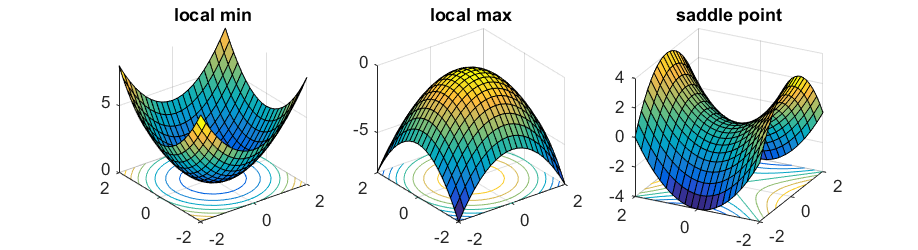
In simpler Machine Learning problems like linear regression with MSE, the loss is a convex quadratic in the parameters, so optimization is well-behaved (a bowl-shaped surface)(e.g. see left in picture).

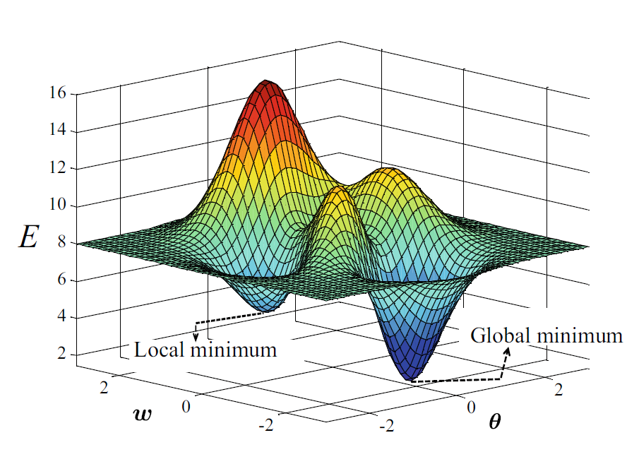
In deep learning, the loss becomes non-convex because it is the result of composing many nonlinear transformations. This creates a complex landscape with saddle points, flat regions, and multiple minima (e.g. see right in picture).

How will Gradient Descent work in this case - non convex function?

Gradient descent does not attempt to find the global minimum, but rather follows the local slope of the cost function and converges to a local minimum or a flat region.

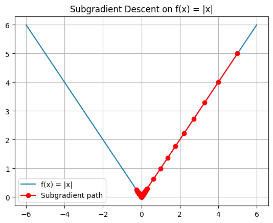
The Loss function is differentiable almost everywhere*. At any point in parameter space, the gradient indicates the direction of steepest local increase, and moving in the opposite direction reduces the cost. During optimization, the algorithm may encounter local minima or saddle points.

(*The function is not differentiable at the point where the function is zero ex ReLU. This is not a problem in practice, as optimization algorithms handle such points using subgradients)

In practice, deep learning works well despite non-convexity, partly because modern networks have millions of parameters and their loss landscapes contain many saddle points and wide, flat minima rather than poor isolated local minima.

Also we rarely use full-batch gradient descent. Instead, we use variants such as Stochastic Gradient Descent (SGD) or mini-batch gradient descent that acts as form of sampling.

In these methods, gradients are computed using a single training example or a small batch of examples rather than the entire dataset.

The resulting gradient is an average over the batch and serves as a noisy approximation of the true gradient. This stochasticity helps the optimizer escape saddle points and sharp minima, enabling effective training in practice.

Next: Backpropagation with Scalar Calculus

References

• Neural Networks and Deep Learning - Michael Nielsen
• Gradient Descent - Wikipedia