The Maths behind Neural Networks
Alex Punnen
© All Rights Reserved
Chapter 3
Gradient Descent and Optimization
A brief history
It is not clear when gradient descent became popular for training neural networks. It is clear that the limitation of Perceptron showed the limitations of shallow layered neural networks. For deeper layers, an effective way of training was the hard part.
Between the perceptron discovery in the late 1960s and the AlexNet Convolutional network in 2012 which ushered the field into the mainstream, neural network architecture,backpropagation algorithm and related techniques were honed to the modern state by many.
If you want a quick look at the some of the known contributors you can start from the reverse mode of automatic differentiation - a mathematical paper around the 1970s by Seppo Linnainmaa. This could have been a base for Geoffrey Hinton, David Rumelhart, Ronald J. Williams paper around 1986 for the backpropagation algorithm for neural network, which inturn could be the base for Yaan Le Cun’s convolutional neural network for handwriting recognition of digits around 1998-2000 Reading Handwritten Digits A Zip Code Recognition System. This could have been the base for Geoffrey Hinton’s student Alex Krizhevsk’s deeper and better Convolutional Neural network ImageNet Classification with Deep Convolutional Neural Networks called AlexNet around 2012. And in 2012 AlexNet left all other ML-based competitors (HOG, HAAR based) far behind in the ImageNet competition.
Beyond this very brief and shallow overview, one needs to refer to a deeper study like Deep Neural Network history Deep Learning in Neural Networks: An Overview Jurgen Schmidhuber and the many people who have contributed. The Wikipedia [history of Backpropagation] shows how many times it has been discovered and re-discovered, from control theory applications to neural nets
Frankly, it does not matter who. It matters how, as it can give an insight into the discovery. But there are quite a lot of overlaps in that short history and quite many brilliant minds contributing, that it is not that linear, to afford us further insight. Suffice it is to say that from 2012 neural network was no more a niche academic field.
Optimization - Newton’s Method and Gradient Descent
Before we go to more complex topics like, let us see the simpler problem, the problem of Optimization of an equation.
Newton’s Method
Before the gradient descent method was invented by Augustin-Louis Cauchy, optimization of a differentiable function was done by Newton’s method, also called Newton -Raphson method possibly for astronomical or orbital solutions.
The intuition regarding this is something like below.
Assume that we need to find the $\sqrt16$. This is the same as solving the equation $x^2 − 16 = 0$. We start with an approximate value and iteratively improve. Assume that $x_0$ is the initial value that we have taken. The derivative of the function at $x_0$ is the slope of the tangent at $x_0$. The main intuition is to take this tangent line intercept at the x-axis as a new point,t and the process is repeated iteratively.
$x_1$ = $x_0$ - $f(x_0)$/$f’(x_0)$
We can see in the figure below where this tangent is touching the x-axis.
$x_1$ = 13.04 for $x_0$=0.628.
We take the tangent at 13.04 and see where that is touching the x-axis (at 7.13)and finally we reach at 4 which is the solution. This is an inflection point of the function.
How does finding the root help in optimization ?
This is because the maximum and minima of the function $f(x)$, happens at $f’(x)$= 0. So we can use the same method as above but instead of solving for $f(x)$=0, we need to solve for $f’(x)$=0.
We can use the same equation and substitute $f’(x)$ instead of $f(x)$.
$x_1$ = $x_0$ - $f’(x_0)$/$f’‘(x_0)$
You can see that in Newton’s method we need to take the second derivative of the function to solve the equation. This makes it more complex than Gradient descent, which only needs the first derivative.
The gradient descent method is much simpler than Newton’s method.

Cost/Loss Function
It is a function which represents the difference between the expected value and the actual value.
\[\begin{aligned} \text{ Say } x_1 \text{is the actual value} \\ \text{Expected value }=\hat x \quad \\ \text{Error in the function} = x_1 -\hat x \\ \end{aligned}\]To make sure that the error is not skewed if the variance is above or below the function, that is positive or negative, we take the square of the difference, and since we are not usually looking at one value, but a set of values, we take the mean of the count of variables. This is the Mean Square Error cost function.
\[{MSE} =\frac {\sum _{i=1}^{n}(X_{i}-{\hat {X_{i}}})^{2}}{n}\]We also have Root Mean Square Error (RMSE)
\[{RMSE} =\sqrt\frac {\sum _{i=1}^{n}(X_{i}-{\hat {X_{i}}})^{2}}{n}\]Where $X_i$ is a vector of calculated values and $\hat X_i$ is the vector of expected values.
MSE is usually for regression problems in ML. For Classification problems, we use Cross-Entropy Loss or Hinge Loss/Multi-class SVM Loss. For Classification loss functions, the output is a probability distribution between 0 and 1.
More details regarding different loss functions here (Different Loss Function)
All the Cost functions used are continuous functions, that is they are differentiable. This is an important feature, as else, we cannot apply gradient descent.
Optimizing the Cost function
Let’s take a closer look at optimizing the cost function. Let’s talk about linear regression (line fitting) ML algorithm and optimizing it using Mean Squared Error via Gradient Descent for a start. This is the simplest to explain visually.
In the diagram below the red line ($y= mx +b$) is the optimal line that one can draw through the sample set. The slope m and constant b is learned by the gradient descent algorithm. The x y-axis could be some data set like house price to area etc, which we have - training data. Once we find a fitting line, we can plugin new values of x to give predicted y values.
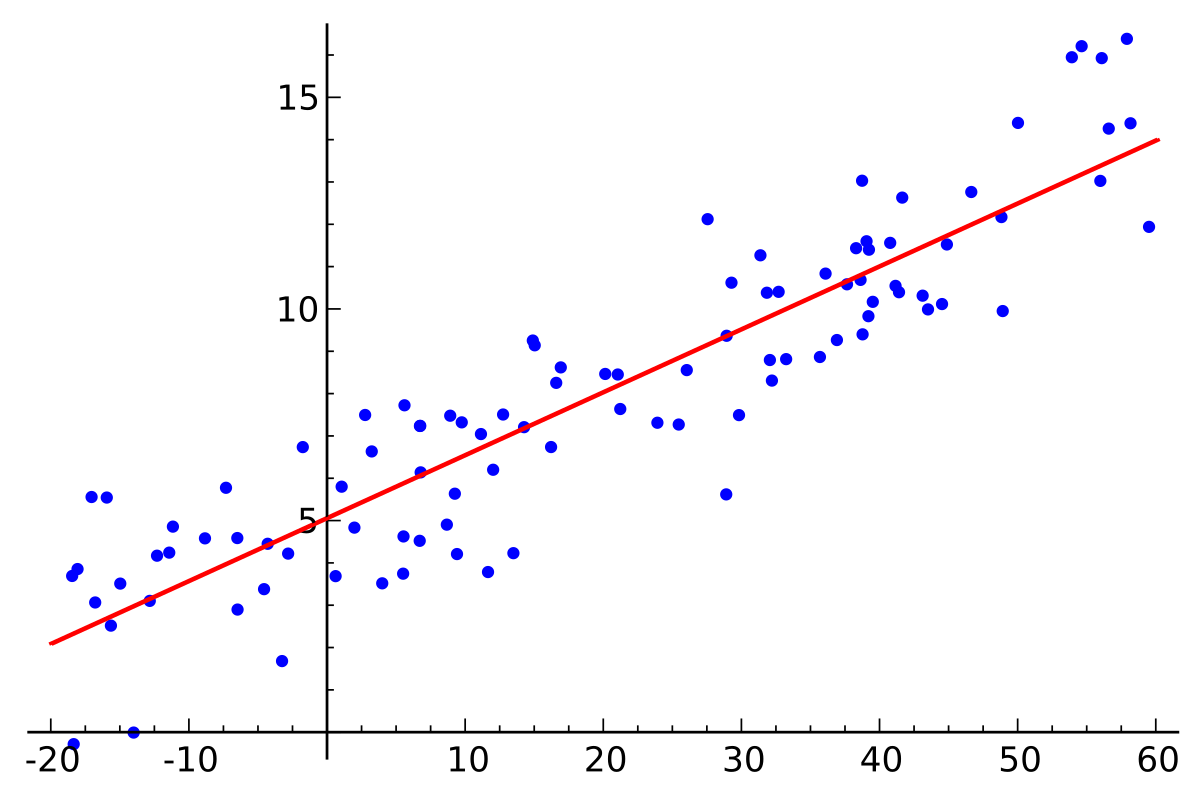
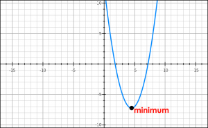
The loss function we use here for regression is a quadratic function (parabolic shape), and the optimal is at the trough.
 source - https://www.analyticsvidhya.com
To explain geometrically,We start at a random point, get the slope of the cost function at the point. The slope or gradient is the derivative of the function at that point ( derivative - the rate of change is also geometrically the slope of a function of two variables. We go towards the negative of the slope (multiplied by a factor called the learning rate)
In the case of MSE, we have just two variables weight and loss, which we can plot as below, and the derivative of the function is simply the geometric slope of the function.

 source - https://developers.google.com/machine-learning/crash-course/reducing-loss/gradient-descent
In case of more complex loss functions with multiple variables, we need to hold one variable constant and take the derivative of the other, and do likewise for all- basically, we need to take the partial derivatives; and arrange these partial derivatives in a matrix; which is the gradient vector, again whose negative gives the direction to take to reach the minimum.
Example for a function $F(x,y,z)$ in three variables, the gradient vector is
\[\begin{bmatrix} \dfrac{ \partial F}{\partial x} \\ \\ \dfrac{\partial F}{\partial y} \\ \\ \dfrac{\partial F}{\partial z} \end{bmatrix}\]And the loss function in say three dimensions will geometrically be something like

But the intuition regarding solving it is the same. Instead of the simple slope as in the case of two-dimensional loss function like MSE, we take the gradient vector and follow the negative to the gradient, with some constant selected as the learning rate. The constant is so chosen, that we decrement in short steps, and reduce the risk of overshooting the minima.