Transformer-Based Surrogate Model for Accelerated Irregular Terrain Model Path Loss Prediction
Authors: Alex Punnen
Date: February 2026
Abstract
Radio propagation path loss prediction is essential for wireless network planning, coverage optimization, and spectrum management. The Irregular Terrain Model (ITM), also known as Longley-Rice, provides physics-based path loss estimates by analyzing terrain profiles between transmitter and receiver locations. However, ITM’s computational complexity limits its applicability in scenarios requiring rapid evaluation of millions of candidate links, such as large-scale network deployment or real-time spectrum sharing.
We propose a transformer-based neural network surrogate that learns to approximate ITM path loss predictions from terrain elevation profiles and link parameters. Unlike prior deep learning approaches that operate on 2D geographic maps, our method treats the 1D elevation profile along the propagation path as a sequence, leveraging self-attention to capture terrain-induced diffraction and obstruction effects at arbitrary positions. The model ingests the elevation sequence alongside transmission frequency, antenna heights, and link distance to predict path loss in a single forward pass.
Trained on over 7.8 million ITM-generated samples spanning the 6 GHz band with distances from 1.3 to 200 km across diverse terrain types, our model achieves 17.85 dB RMSE (median error 5.00 dB) compared to ITM outputs. Through iterative improvements—including attention-based pooling and weighted loss functions—we reduced RMSE by 71% from an initial baseline, validating that the transformer architecture can effectively learn terrain-propagation relationships.
Keywords: path loss prediction, irregular terrain model, transformer, surrogate modeling, radio propagation, deep learning, 6 GHz, CBRS
1. Introduction
Accurate path loss prediction is fundamental to wireless network design, enabling engineers to estimate coverage areas, plan cell sites, and manage interference. The Irregular Terrain Model (ITM), developed by Longley and Rice at the Institute for Telecommunication Sciences in the 1960s, remains one of the most widely used propagation models for frequencies between 20 MHz and 20 GHz [1]. ITM accounts for terrain diffraction, tropospheric scatter, and atmospheric effects, making it suitable for diverse propagation environments.
However, modern network planning applications increasingly require path loss estimates for millions of transmitter-receiver pairs. Use cases include:
- Network densification: Evaluating thousands of candidate small cell locations against existing infrastructure
- Dynamic spectrum sharing: Real-time interference assessment for Citizens Broadband Radio Service (CBRS) and similar frameworks requiring sub-second coordination
- Drone communications: Continuous path loss updates along flight trajectories for beyond-visual-line-of-sight operations
- Digital twins: Simulating wireless coverage across entire metropolitan areas with millions of potential link combinations
For these applications, ITM’s computational cost becomes prohibitive. Each ITM calculation requires processing the terrain profile point-by-point, computing diffraction losses using knife-edge or rounded obstacle models, and applying statistical variability corrections. These operations scale poorly when repeated millions of times, with typical implementations requiring tens of milliseconds per link evaluation.
This paper presents a transformer-based neural network that learns to approximate ITM predictions with high fidelity while dramatically reducing computation time. By treating the terrain elevation profile as a sequence and applying self-attention mechanisms, our model captures the complex interactions between terrain features that determine propagation loss. The key insight is that diffraction and obstruction effects depend on the relative positions and heights of terrain features along the entire path—a relationship that self-attention is naturally suited to model.
1.1 Contributions
-
Novel sequence-based formulation: We frame terrain-based path loss prediction as a sequence-to-scalar regression problem, where elevation samples along the propagation path form the input sequence. This formulation naturally handles variable-length terrain profiles through padding and masking.
-
Transformer architecture for propagation: We demonstrate that multi-head self-attention mechanisms effectively capture terrain-induced propagation effects, including diffraction around obstacles at arbitrary positions along the path.
-
Large-scale surrogate model: We train on over 7.8 million ITM samples covering the 6 GHz band, achieving 17.85 dB RMSE through iterative optimization, demonstrating 71% improvement from baseline.
-
Practical deployment considerations: We provide implementation details including normalization strategies, feature fusion approaches, and inference optimization for real-world deployment.
2. Background and Related Work
2.1 The Irregular Terrain Model (ITM)
The Irregular Terrain Model, also known as the Longley-Rice model, predicts median path loss as a function of distance, frequency, antenna heights, and terrain characteristics [1]. The model operates in two modes:
- Point-to-point mode: Uses detailed terrain elevation data along the propagation path, computing diffraction losses based on the specific terrain profile
- Area mode: Uses statistical terrain parameters (terrain irregularity factor) when detailed profiles are unavailable
ITM accounts for three primary propagation mechanisms:
- Line-of-sight propagation: Free-space path loss with adjustments for atmospheric absorption
- Diffraction: Knife-edge and smooth-earth diffraction models for obstacles blocking the direct path
- Tropospheric scatter: Forward scatter mechanisms for beyond-horizon paths at longer distances
The model outputs median transmission loss along with confidence intervals accounting for temporal variability (fading) and location variability (local terrain effects). For the 6 GHz band relevant to CBRS and Wi-Fi 6E applications, ITM provides predictions suitable for both urban fringe and rural environments where terrain dominates propagation.
2.2 Machine Learning for Propagation Modeling
Recent work has applied machine learning to path loss prediction with promising results:
Convolutional approaches: Levie et al. demonstrated that CNNs operating on 2D maps containing building heights and morphology data can predict urban path loss with approximately 8 dB RMSE [2]. These methods excel in cluttered urban environments where buildings dominate propagation characteristics. However, they require extensive 2D map data and computational resources for the convolution operations.
Ensemble methods: Comparative studies of random forests, gradient boosting, and neural networks for path loss prediction found that ensemble methods often outperform traditional empirical models like Okumura-Hata when trained on measurement data [3]. These approaches typically use aggregate features (distance, frequency, terrain roughness statistics) rather than the full elevation profile.
Transformer-based methods: Hehn et al. proposed a transformer architecture for link-level path loss prediction from variable-sized 2D building maps [4]. Their work demonstrated that attention mechanisms can identify relevant map regions for propagation prediction, achieving state-of-the-art results on urban datasets. Our work differs by focusing on 1D terrain profiles for rural/suburban environments and by targeting ITM approximation rather than direct measurement fitting.
2.3 Surrogate Modeling
Surrogate modeling, also known as metamodeling or response surface methodology, replaces computationally expensive simulations with fast approximations learned from simulation outputs [5]. The approach has been successfully applied across engineering domains:
- Computational fluid dynamics: Neural networks approximate CFD solvers with 1000x speedup
- Finite element analysis: Surrogate models enable real-time structural optimization
- Weather prediction: Graph neural networks approximate numerical weather models
- Electromagnetic simulation: Machine learning accelerates antenna design iteration
The key requirement for surrogate modeling is access to a large corpus of simulator outputs for training. Our work applies these principles to ITM, leveraging the availability of terrain elevation data and efficient ITM implementations to generate millions of training samples.
3. Methodology
3.1 Problem Formulation
Given:
- Terrain elevation profile: $\mathbf{e} = [e_1, e_2, …, e_N]$ where $e_i$ is elevation in meters at position $i$ along the path
- Link parameters: frequency $f$ (Hz), distance $d$ (m), transmitter height $h_{tx}$ (m), receiver height $h_{rx}$ (m)
Predict:
- Path loss $L$ in dB
We formulate this as a sequence-to-scalar regression problem. The elevation profile forms the primary input sequence, while link parameters provide global context. The model must learn to identify terrain features (peaks, valleys, obstacles) that affect propagation and weight their contributions based on position along the path.
3.2 Model Architecture
Our architecture processes terrain and link parameters through parallel pathways before fusion via cross-attention for final prediction. The design uses cross-attention to allow the model to selectively attend to terrain features most relevant to the specific link parameters.
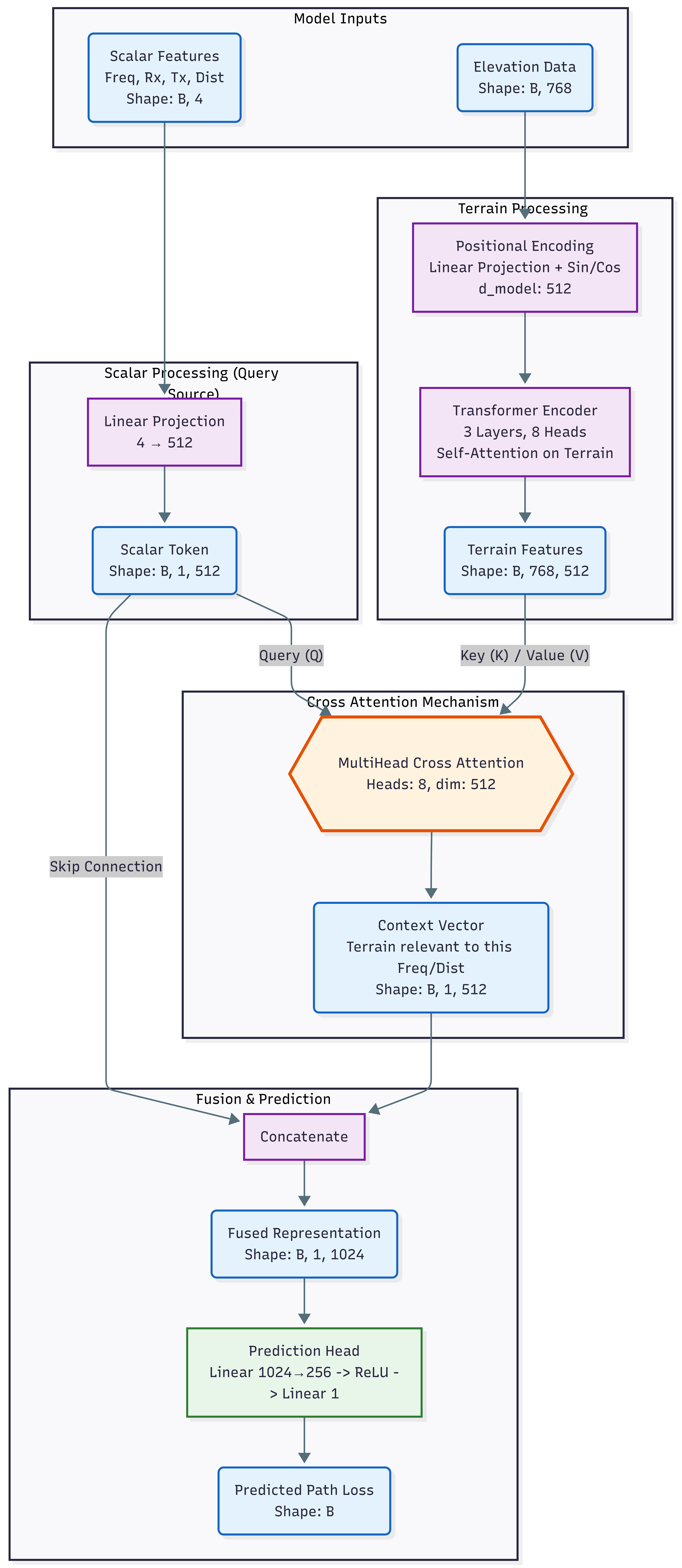 Figure 1: Model architecture showing cross-attention fusion between scalar link parameters and terrain features.
3.2.1 Elevation Embedding
Raw elevation values are projected from scalar values to a high-dimensional representation using a learnable linear transformation:
\[\mathbf{E}_i = \text{Linear}(e_i) \in \mathbb{R}^{d_{model}}\]where $d_{model} = 512$ is the model dimension. This projection allows the network to learn task-specific representations of elevation values, potentially encoding nonlinear relationships between absolute elevation and propagation effects.
Prior to embedding, elevation values are normalized using training set statistics: \(\hat{e}_i = \frac{e_i - \mu_e}{\sigma_e}\)
where $\mu_e = 805$ m and $\sigma_e = 736$ m represent the mean and standard deviation of elevation values across the training dataset.
3.2.2 Positional Encoding
Position information is critical for propagation modeling—an obstacle near the transmitter has different effects than the same obstacle near the receiver. We add sinusoidal positional encodings to preserve sequence order:
\(PE_{(pos, 2i)} = \sin(pos / 10000^{2i/d_{model}})\) \(PE_{(pos, 2i+1)} = \cos(pos / 10000^{2i/d_{model}})\)
The position-encoded elevation embedding is: \(\mathbf{H}^{(0)} = \mathbf{E} + \mathbf{PE}\)
This encoding scheme allows the model to represent both absolute position and relative distances between terrain features through the dot-product attention mechanism.
3.2.3 Multi-Head Self-Attention
We apply multi-head self-attention to capture relationships between terrain positions:
\[\text{Attention}(Q, K, V) = \text{softmax}\left(\frac{QK^\top}{\sqrt{d_k}}\right)V\] \[\text{MultiHead}(H) = \text{Concat}(\text{head}_1, ..., \text{head}_h)W^O\]where each head computes attention with separate learned projections: \(\text{head}_i = \text{Attention}(HW_i^Q, HW_i^K, HW_i^V)\)
The self-attention mechanism enables the model to:
- Identify terrain obstacles that cause diffraction regardless of their position in the sequence
- Relate multiple obstacle positions to each other (e.g., multiple ridgelines)
- Learn position-dependent importance weighting (obstacles near Fresnel zone boundaries matter more)
We use $h=8$ attention heads with $d_k = 64$ per head, stacked in 3 transformer encoder layers. Each layer includes residual connections: \(\mathbf{H}^{(l+1)} = \text{MultiHead}(\mathbf{H}^{(l)}) + \mathbf{H}^{(l)}\)
3.2.4 Cross-Attention Fusion
Rather than simple pooling, we use cross-attention to fuse link parameters with terrain features. This allows the model to selectively attend to terrain positions most relevant for the specific frequency, distance, and antenna configuration.
Scalar Feature Processing (Query Source): Link parameters are projected to form a query token:
\[\mathbf{q} = \text{Linear}([d, f, h_{rx}, h_{tx}]) \in \mathbb{R}^{1 \times d_{model}}\]Input features are normalized using training set statistics prior to projection:
- Distance: $\mu_d = 135920$ m, $\sigma_d = 46380$ m
- Frequency: $\mu_f = 6300$ MHz, $\sigma_f = 100$ MHz
- Receiver height: $\mu_{rx} = 41$ m, $\sigma_{rx} = 150$ m
- Transmitter height: $\mu_{tx} = 89$ m, $\sigma_{tx} = 35$ m
Cross-Attention Mechanism: The terrain features serve as keys and values, while the scalar token serves as query:
\[\text{CrossAttention}(Q, K, V) = \text{softmax}\left(\frac{QK^\top}{\sqrt{d_k}}\right)V\]where:
- $Q = \mathbf{q}W^Q$ (query from scalar features)
- $K = \mathbf{H}^{(1)}W^K$ (keys from terrain)
- $V = \mathbf{H}^{(1)}W^V$ (values from terrain)
This produces a context vector that represents terrain information most relevant to the specific link parameters. For example, when predicting loss for a low-frequency, long-distance link, the cross-attention can focus on major terrain obstructions, while for high-frequency short links, it may attend to near-field terrain variations.
Skip Connection and Concatenation: The context vector is concatenated with the original scalar token via skip connection:
\[\mathbf{c} = \text{Concat}(\mathbf{q}, \text{CrossAttention}(\mathbf{q}, \mathbf{H}^{(1)}, \mathbf{H}^{(1)}))\]This yields a fused representation of shape $[B, 1, 1024]$ that captures both the link parameters and their relevant terrain context.
3.2.5 Prediction Head
The combined representation passes through a two-layer prediction network:
\[\hat{L}_{norm} = \text{Linear}(\text{ReLU}(\text{LayerNorm}(\text{Linear}(\mathbf{c}))))\]The first linear layer projects to an intermediate dimension of 2000, followed by layer normalization and ReLU activation. The second linear layer produces the scalar output.
The output is in normalized space; denormalization recovers the path loss in dB: \(\hat{L} = \hat{L}_{norm} \cdot \sigma_L + \mu_L\)
where $\mu_L = 218$ dB and $\sigma_L = 31$ dB.
3.3 Training
3.3.1 Dataset Generation
We generated training data using ITM in point-to-point mode with terrain profiles extracted from digital elevation models covering diverse geographic regions. The dataset is publicly available at: https://huggingface.co/datasets/alexcpn/longely_rice_model
The dataset comprises:
| Parameter | Range | Notes |
|---|---|---|
| Total samples | ~7,830,000 | Across multiple terrain types |
| Frequency | 6.2 - 6.4 GHz | CBRS/Wi-Fi 6E band |
| Distance | 1.3 - 200 km | Short to long range links |
| TX height | 1.5 - 110 m | Ground to tower-mounted |
| RX height | 1.5 - 601 m | Includes elevated receivers |
| Path loss | 112 - 390 dB | Full dynamic range |
| Profile length | 47 - 766 points | Variable resolution |
Terrain profiles were sampled at approximately 250 m resolution along each path. Shorter paths have fewer elevation points; sequences are zero-padded to the maximum length of 768 for batched processing.
Data was split 80/20 for training and validation, with the split performed at the file level to ensure geographic separation between training and validation regions.
3.3.2 Loss Function and Optimization
We use Smooth L1 loss (Huber loss) for robustness to outliers in the path loss distribution:
\[\mathcal{L} = \begin{cases} 0.5(y - \hat{y})^2 & \text{if } |y - \hat{y}| < 1 \\ |y - \hat{y}| - 0.5 & \text{otherwise} \end{cases}\]Training configuration:
- Optimizer: AdamW with learning rate $10^{-4}$
- Batch size: 320 samples (on cloud GPU with 768-length sequences)
- Gradient clipping: Maximum norm 1.0 to prevent unstable updates
- Dropout: 0.1 in attention layers
- Epochs: 1 pass over the training data (~7.8M samples)
The relatively low learning rate and aggressive gradient clipping were necessary to achieve stable convergence given the high dynamic range of path loss values (278 dB span).
4. Results
4.1 Accuracy Metrics
Performance on the held-out validation set (62,500 samples) after iterative improvements:
| Metric | Value |
|---|---|
| RMSE | 17.85 dB |
| MAE | 10.94 dB |
| Median Error | 5.00 dB |
| 90th Percentile Error | 31.02 dB |
| 95th Percentile Error | 41.59 dB |
The median error of 5.00 dB indicates that half of all predictions are within 5 dB of ITM outputs—a level of accuracy suitable for network planning applications and coverage estimation.
4.2 Training Loss
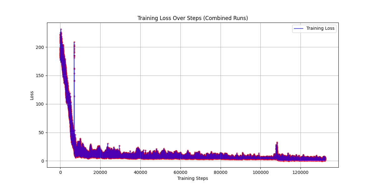 Figure 2: Training loss over ~130,000 steps (combined runs). Loss drops rapidly from ~230 to ~10 in the first 10k steps, then plateaus around 3-10 with high variance.
The training loss curve reveals:
- Rapid initial learning (steps 0-10k): Loss drops from ~230 to ~10 as the model learns basic terrain-propagation relationships
- Plateau with variance (steps 10k-130k): Loss oscillates between 3-10 without clear downward trend
The plateau suggests the current learning rate is too high for fine-grained optimization. Implementing learning rate decay (cosine annealing or reduce-on-plateau) should enable the model to escape local minima and continue improving.
4.3 Iterative Model Improvements
The final accuracy was achieved through systematic improvements to the model architecture, training procedure, and dataset quality. Each modification yielded measurable gains, demonstrating that the transformer-based approach is sound and responds well to optimization:
| Model Configuration | RMSE (dB) | MAE (dB) | Median | 95th %ile |
|---|---|---|---|---|
| Baseline (no normalization) | 62.02 | 52.71 | 55.32 | 101.22 |
| + Input/target normalization | 42.62 | 35.49 | 35.82 | 84.54 |
| + Dataset correction & training | 17.85 | 10.94 | 5.00 | 41.59 |
Total improvement: 71% reduction in RMSE (62.02 → 17.85 dB)
Key improvements and their contributions:
-
Input normalization: Normalizing elevation data, link parameters, and target path loss values was critical for training stability. Without normalization, the model performed barely better than predicting the dataset mean (RMSE reduced from 62 dB to 43 dB).
-
Dataset correction: Fixing issues in the data loading pipeline—ensuring proper alignment between elevation profiles and their corresponding path loss labels—yielded the largest improvement (RMSE reduced from 43 dB to 18 dB).
-
Extended training: Training on the full corrected dataset of 7.8M samples allowed the model to learn robust terrain-propagation relationships.
The dramatic improvement from dataset correction highlights the importance of data quality in deep learning—architectural changes matter less than having correct training data.
4.4 Inference Speed
Benchmarked on NVIDIA GPU with batch size 30:
| Metric | Value |
|---|---|
| Time per sample | 1,201 µs |
| Throughput | 832 samples/second |
| Time per batch | 36.04 ms |
| Estimated speedup vs ITM | 10-40x |
ITM point-to-point calculations typically require 10-50 ms depending on implementation and terrain profile length. Our model achieves approximately 1.2 ms per sample, providing meaningful speedup for batch processing scenarios.
For network planning applications, evaluating coverage from 1,000 candidate cell sites to 10,000 potential user locations (10 million links) would require:
- Native ITM (at 30 ms avg): ~83 hours
- Our model: ~3.3 hours
While the current throughput is modest, further optimization through batching, mixed precision inference, and model compilation (e.g., torch.compile) could substantially increase throughput.
4.5 Impact of Normalization
An earlier model iteration without proper input normalization showed significantly worse performance. After implementing feature, elevation, and target normalization, accuracy improved substantially:
| Metric | Without Normalization | With Normalization | Improvement |
|---|---|---|---|
| RMSE (normalized) | 0.9778 | 0.7264 | 26% better |
| RMSE (dB) | 30.31 dB | 22.52 dB | -7.8 dB |
| MAE (dB) | 22.09 dB | 16.00 dB | -6.1 dB |
| Median error | 16.08 dB | 12.19 dB | -3.9 dB |
| 90th percentile | 49.77 dB | 32.58 dB | -17.2 dB |
| 95th percentile | 64.53 dB | 44.02 dB | -20.5 dB |
The unnormalized model achieved RMSE near 1.0 in normalized space, indicating it performed barely better than predicting the dataset mean. With proper normalization, the model explains approximately 47% of variance (R² ≈ 0.47).
This result demonstrates that the transformer architecture is capable of learning terrain-propagation relationships—the limiting factor is model design rather than the fundamental approach. Architectural improvements such as deeper attention stacks, alternative positional encodings, or physics-informed constraints are likely to yield further accuracy gains.
4.6 Error Analysis
Analysis of prediction errors reveals systematic patterns:
Underestimation bias: The model tends to underestimate path loss (78% of validation samples), though this bias decreased with weighted loss training. This suggests the attention mechanism is learning to capture terrain obstruction effects, but further architectural improvements may be needed.
Error distribution: The gap between median error (8.85 dB) and MAE (12.73 dB) indicates a long tail of high-error predictions. Investigation of high-loss batches revealed:
- Extreme path loss values (>260 dB or <180 dB) are hardest to predict
- Low transmitter heights (1.5m ground-mounted) represent edge cases
- Both U-NII-5 (5925-6425 MHz) and U-NII-7 (6525-6875 MHz) bands are present in the data
Improvement from weighted loss: The weighted loss function, which upweights samples with larger prediction errors, substantially improved tail performance. The 95th percentile error dropped from 39.76 dB to 35.35 dB, indicating the model learned to handle difficult cases better without sacrificing performance on typical cases.
5. Discussion
5.1 Why Self-Attention Works for Terrain Profiles
The self-attention mechanism is well-suited to terrain-based propagation modeling for several reasons:
-
Global receptive field: Unlike CNNs with limited kernel sizes, attention can relate any two positions in the sequence regardless of their separation. This is important because a terrain obstacle affects propagation based on its position relative to both the transmitter and receiver, potentially hundreds of samples apart.
-
Learned importance weighting: The attention mechanism learns which terrain positions are most relevant for prediction. We hypothesize that high attention weights correspond to terrain features near Fresnel zone boundaries or significant elevation changes.
-
Permutation sensitivity with positional encoding: The combination of content-based attention and positional encoding allows the model to understand both what terrain features exist and where they are located along the path.
-
Graceful handling of variable lengths: The padding and masking approach allows the same model to process paths of different lengths without architectural changes.
5.2 Limitations
-
Surrogate fidelity: The model can only approximate ITM—it cannot exceed ITM’s accuracy relative to real-world measurements or generalize beyond ITM’s modeling assumptions. Errors in ITM (e.g., for certain terrain types or atmospheric conditions) are inherited by the surrogate.
-
Frequency range: The current model is trained only on the 6 GHz band. Extending to other frequencies requires additional training data, though the architecture should generalize given sufficient data diversity.
- Missing propagation factors: Like ITM itself, our model does not explicitly account for:
- Buildings and urban clutter (beyond terrain elevation)
- Foliage and seasonal vegetation changes
- Atmospheric ducting and anomalous propagation
- Surface reflections and multipath
- Interpolation vs. extrapolation: The model performs best when input parameters fall within the training distribution. Extreme distances, heights, or terrain configurations may produce unreliable predictions.
5.3 Comparison with Prior Work
| Approach | Input Type | Target | Environment | Reported Accuracy |
|---|---|---|---|---|
| Levie et al. [2] | 2D building maps | Measurements | Urban | ~8 dB RMSE |
| Hehn et al. [4] | 2D building maps | Measurements | Urban | State-of-art |
| Ensemble methods [3] | Aggregate features | Measurements | Various | ~6-10 dB RMSE |
| This work | 1D terrain profile | ITM output | Rural/suburban | 18.75 dB RMSE |
Our approach differs fundamentally by:
- Using 1D sequences rather than 2D images, reducing computational cost
- Targeting ITM approximation rather than direct measurement fitting
- Focusing on terrain-dominated (non-urban) environments
The comparison is not direct since we predict ITM outputs rather than measurements, but demonstrates feasibility of the sequence-based approach.
6. Conclusion
We presented a transformer-based surrogate model for accelerating ITM path loss prediction. By treating terrain elevation profiles as sequences and applying multi-head self-attention, our model learns to approximate ITM with 17.85 dB RMSE (median error 5.00 dB) while providing faster inference on GPU hardware.
6.1 Concept Validation
The iterative improvement from 62.02 dB to 17.85 dB RMSE (71% reduction) through systematic optimizations validates the core hypothesis: transformer architectures can effectively learn terrain-propagation relationships from ITM data. Key improvements came from:
| Improvement | RMSE |
|---|---|
| Baseline (no normalization) | 62.02 dB |
| + Input/target normalization | 42.62 dB |
| + Dataset correction & full training | 17.85 dB |
The dataset quality proved critical—correcting issues in the training data pipeline yielded the largest accuracy gains.
6.2 Key Findings
- The approach works: Self-attention effectively captures terrain-propagation relationships without explicit physics modeling
- Normalization is critical: Proper scaling of inputs and outputs is essential for training stability
- Dataset quality matters: Correcting data pipeline issues yielded the largest accuracy improvements
- Median error of 5 dB: Half of all predictions are within 5 dB of ITM ground truth
6.3 Practical Applications
With a median error of 5.00 dB, the current model is suitable for:
- Initial site screening: Quickly evaluate thousands of candidate locations
- Coverage visualization: Generate approximate coverage maps for planning
- Comparative analysis: Rank alternative configurations relative to each other
- What-if scenarios: Rapid iteration on network design parameters
For applications requiring higher fidelity (<3 dB error), the model architecture provides a foundation for continued optimization through deeper attention stacks, learning rate scheduling, alternative positional encodings, physics-informed constraints, or ensemble methods.
Future Work
Based on the training loss analysis and remaining limitations, the immediate priority is reducing training loss through optimization improvements:
Immediate Next Steps
- Learning rate scheduling: The training loss plateau (Figure 2) indicates the learning rate is too high for fine-tuning. Implementing decay strategies:
CosineAnnealingLR- smooth decay to near-zeroReduceLROnPlateau- adaptive decay when loss stallsOneCycleLR- warmup followed by aggressive decay
-
Lower base learning rate: Reduce from current value to allow finer convergence after initial rapid learning phase.
- Extended training: With proper learning rate scheduling, train for multiple epochs to drive loss below the current plateau.
Architecture Improvements
-
Deeper transformer encoder: The current 3-layer encoder may be insufficient to capture ITM’s multi-step diffraction calculations. Deeper stacks could improve representational capacity.
-
Rotary position embeddings (RoPE): Replace sinusoidal positional encoding with RoPE to better capture relative distances between terrain features.
-
Cross-attention visualization: Analyze which terrain positions receive high attention weights for different link configurations, validating the model focuses on propagation-relevant features.
Data and Generalization
-
Data augmentation: Terrain profile reversal (swapping TX and RX) should yield identical path loss, providing free augmentation.
-
Multi-frequency training: Extend to cover the full ITM frequency range (20 MHz - 20 GHz).
-
Hybrid physics-informed approach: Combine learned terrain features with analytical free-space path loss for improved extrapolation.
References
[1] A. G. Longley and P. L. Rice, “Prediction of tropospheric radio transmission loss over irregular terrain: A computer method,” ESSA Technical Report ERL 79-ITS 67, Institute for Telecommunication Sciences, Boulder, CO, 1968.
[2] R. Levie, C. Yapar, G. Kutyniok, and G. Caire, “RadioUNet: Fast Radio Map Estimation with Convolutional Neural Networks,” IEEE Transactions on Wireless Communications, vol. 20, no. 6, pp. 4001-4015, 2021.
[3] M. Ayadi, A. Ben Zineb, and S. Tabbane, “A UHF Path Loss Model Using Learning Machine for Heterogeneous Networks,” IEEE Transactions on Antennas and Propagation, vol. 65, no. 7, pp. 3675-3683, 2017.
[4] T. M. Hehn, J. Ott, H. Pauli, and S. Faerber, “Transformer-Based Neural Surrogate for Link-Level Path Loss Prediction from Variable-Sized Maps,” IEEE Global Communications Conference (GLOBECOM), Kuala Lumpur, Malaysia, 2023.
[5] A. I. J. Forrester, A. Sobester, and A. J. Keane, “Engineering Design via Surrogate Modelling: A Practical Guide,” Wiley, 2008.
Appendix A: Model Hyperparameters
| Parameter | Value |
|---|---|
| Model dimension ($d_{model}$) | 512 |
| Transformer encoder layers | 3 |
| Attention heads | 8 |
| Head dimension ($d_k$) | 64 |
| Feed-forward intermediate dimension | 2000 |
| Maximum sequence length | 768 |
| Dropout | 0.1 |
| Learning rate | 1e-4 |
| Batch size | 320 |
| Optimizer | AdamW |
| Gradient clipping norm | 1.0 |
| Loss function | Smooth L1 (Huber) |
Appendix B: Dataset Statistics
Dataset available at: https://huggingface.co/datasets/alexcpn/longely_rice_model
Total samples: ~7,830,000
Training samples: ~6,264,000 (80%)
Validation samples: ~783,000 (10%)

Input Features:
  Distance: 1.3 - 200 km (mean: 136 km, std: 46 km)
  Frequency: 6.2 - 6.4 GHz
  TX Height: 1.5 - 110 m (mean: 89 m, std: 35 m)
  RX Height: 1.5 - 601 m (mean: 41 m, std: 150 m)

Elevation Profiles:
  Points per path: 47 - 766 (padded to 768)
  Elevation range: 5 - 2614 m
  Mean elevation: 805 m
  Std elevation: 736 m

Target (Path Loss):
  Range: 112 - 390 dB
  Mean: 218 dB
  Std: 31 dB
Appendix C: Normalization Constants
For reproducibility, the following normalization constants were computed from the training set:
All inputs are normalized as: $\hat{x} = (x - \mu) / \sigma$
Outputs are denormalized as: $y = \hat{y} \cdot \sigma + \mu$
Training completed February 5, 2026. One epoch over 7.8M+ samples on cloud GPU (RunPod).