Perceptron Training via Feature Vectors & HyperPlane split
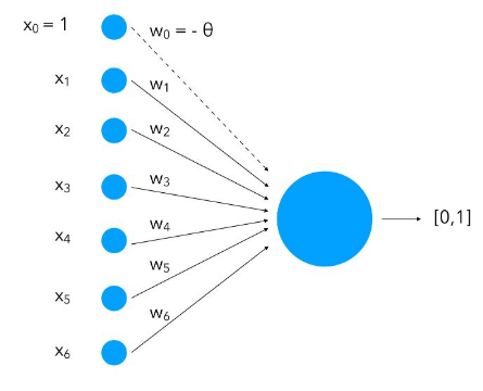
Let’s follow from the previous chapter of the Perceptron neural network.
We have seen how the concept of splitting the hyper-plane of feature set separates one type of feature vectors from other.
How are the weights learned?
You may have heard about Gradient Descent, which is the backbone of training modern neural networks. However, for the classic Perceptron, the learning algorithm is much simpler and relies on a geometric intuition.
The goal is to find a weight vector $w$ that defines a hyperplane separating the two classes of data (e.g., Positive and Negative).
Note this term hyperplane is used in the context of feature vector space and is used throughout neural network learning.
The Intuition: Nudging the Vector
Imagine the weight vector $w$ as a pointer. We want this pointer to be oriented such that:
- It points generally in the same direction as Positive examples.
- It points away from Negative examples.
We start with a random weight vector. Then, we iterate through our training data and check how the current $w$ classifies each point.
- If the classification is correct: We do nothing. The weight vector is already doing its job for this point.
- If the classification is wrong: We need to “nudge” or rotate the weight vector to correct the error.
The Update Rules
Let’s say we have an input vector $x$.
Case 1: False Negative The input $x$ is a Positive example ($y=1$), but our current $w$ classified it as negative (dot product $w \cdot x < 0$).
- Action: We need to rotate $w$ towards $x$.
- Update: $w_{new} = w_{old} + x$
- Result: Adding $x$ to $w$ makes the new vector more aligned with $x$, increasing the dot product for the next time.
Case 2: False Positive The input $x$ is a Negative example ($y=0$ or $-1$), but our current $w$ classified it as positive (dot product $w \cdot x > 0$).
- Action: We need to rotate $w$ away from $x$.
- Update: $w_{new} = w_{old} - x$
- Result: Subtracting $x$ from $w$ pushes it in the opposite direction, decreasing the dot product.
The Formal Algorithm
We can combine these rules into a single update equation. We often introduce a learning rate $\eta$ (a small number like 0.1) to make the updates smoother, preventing the weight vector from jumping around too wildly.
For each training example $(x, y_{target})$:
- Compute prediction: $\hat{y} = \text{step_function}(w \cdot x)$
- Calculate error: $error = y_{target} - \hat{y}$
- Update weights: \(w = w + \eta \cdot error \cdot x\)
This is known as the Perceptron Learning Rule.
\[\Delta w_j = \eta (y_{target} - \text{prediction}) x_j\]Note: This is distinct from Gradient Descent. Gradient Descent requires a differentiable activation function to compute gradients (slope). The Perceptron uses a “step function” (hard 0 or 1) which is not differentiable. However, this simple rule is guaranteed to converge if the data is linearly separable.
A more rigorous explanation of the proof can be found in the book Neural Networks by R.Rojas or this article.
Next: Gradient Descent and Optimization